
Second of two posts about KoggerApp. The was about what the application draws — echogram, bathymetry, side-scan mosaic and the map. This one is about the rest of the sonar survey workflow: the workspace you arrange, the tools you measure with, the devices feeding it all, and the files you hand to someone else. It is a tour rather than a manual — what exists and why it is there.
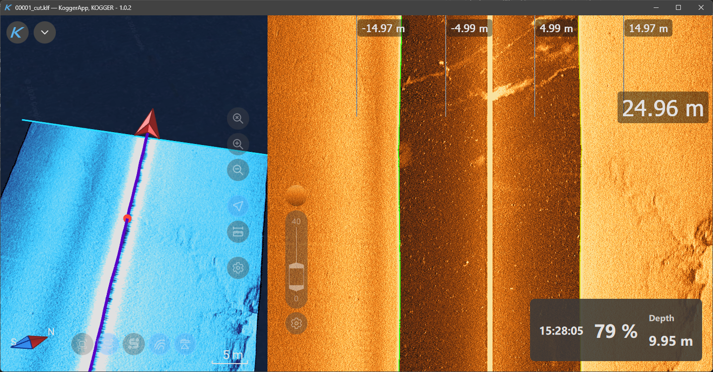
Main window during a survey
The workspace
The application is built to be rearranged rather than learned — the screen you want while running a line is rarely the screen you want while reviewing what you just passed over.
Panes and layouts
The window is a tree of panes. Split it and give each pane a mode — 3D scene, echogram, and so on. Move the border between two panes by grabbing it and pulling, or double-click a pane to throw it out to the full window and double-click again to put it back.
The same survey reads differently depending on how you look at it. Switch a pane’s mode and the measurement is in front of you from another angle — convenient in hydrography, and it costs nothing: nothing to open, no place to lose.
Arrangements that work are worth keeping, and different jobs want different ones. Layouts save them and switch from a menu with snapshot previews, so you pick one by its shape rather than by its name. The ones you use daily go to favourites. On a tablet the layout rotates into a form built for portrait, not a squeezed desktop.
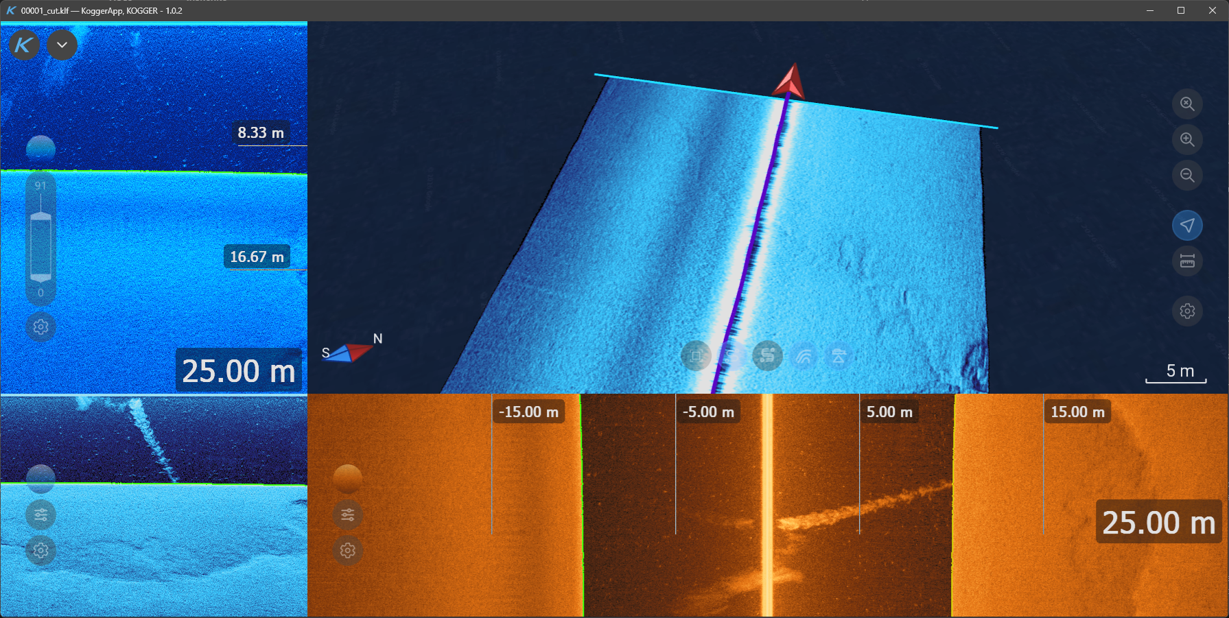
Workspace with 4 panes
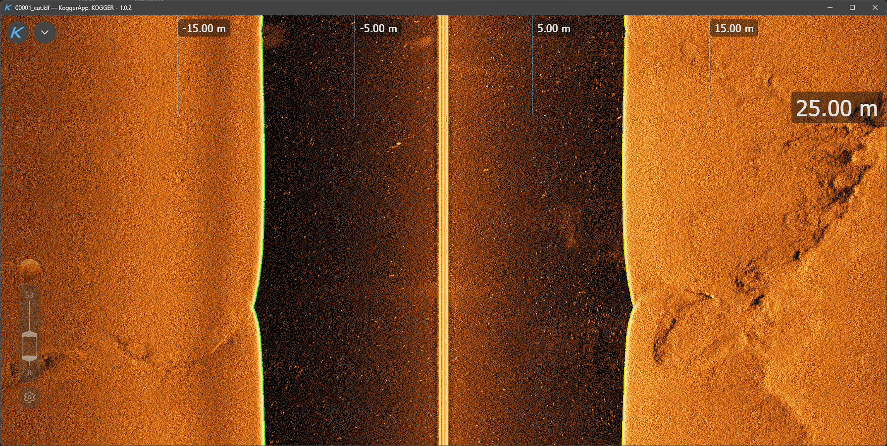
Single-echogram workspace
Two monitors at the helm are wasted on two half-screens. What you usually want is one screen showing one thing, as large as it goes.
A second application window does that: the 3D scene filling one monitor, the echogram filling the other, both live, both resizing smoothly while data keeps coming. Everything else stays out of the way in the main window.
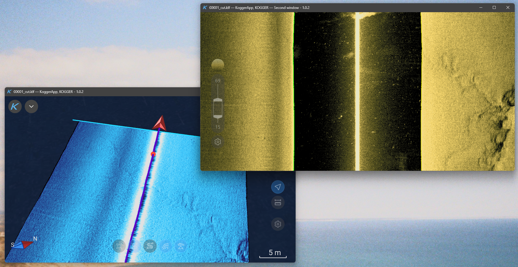
Second window
Floating pop-ups
Attention belongs on the measurement. Everything else should be visible without competing for the same space.
That is what the pop-ups are for: the echogram keeps the screen and your attention, while the boat’s track floats in a small 3D window in the corner where you can glance at it. Tool panels behave like windows — drag, resize, snap to edges — and a pop-up can go fullscreen inside its pane when you do need to look properly, or global, floating above the whole application so it stays with you no matter which pane you switch to.
Open several and they push each other into free space instead of stacking. Resize the app, dock it, plug in a second monitor — they come back where you left them.
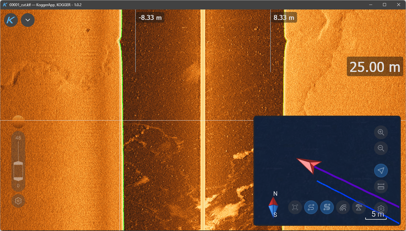
3d scene pop-up
Quick actions
Every survey comes down to a handful of actions you repeat all day — and which ones depends entirely on the job and the rig. There is no default that fits everyone, so the menu is yours to build: toggle items on and off, drag to reorder, and they wrap into rows as you add more. Put what your day is made of within thumb’s reach and leave the rest in the settings page.
The available items cover logging, connected devices, profiles, layouts, widget panels, bottom-track editing, the second window and the console.
Some of them are more than buttons. The logging pill starts and stops recording and shows state and duration inline; the device pill changes sonar frequency without opening settings at all. The same one-tap actions also appear on settings-group headers, next to the settings they belong to.
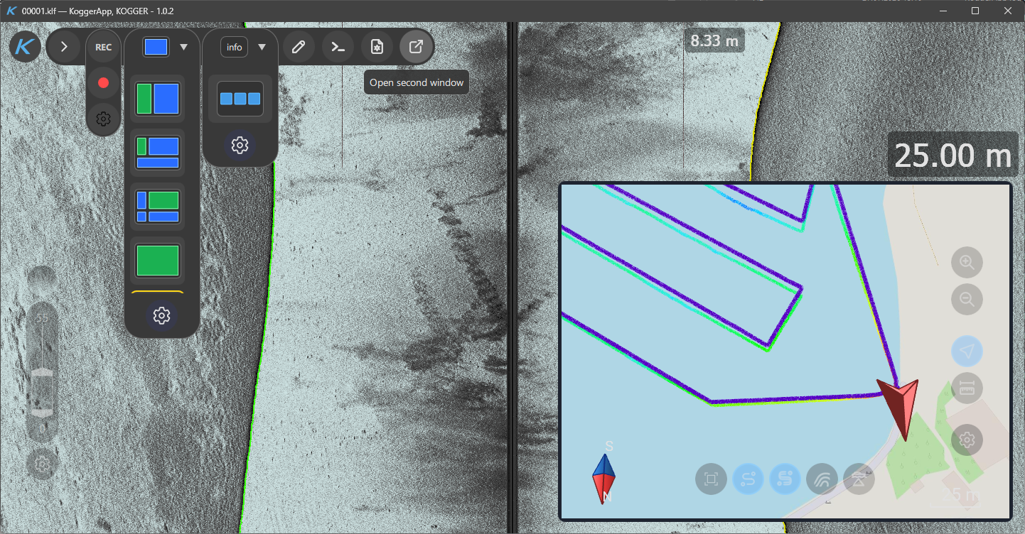
Quick actions
Data widgets
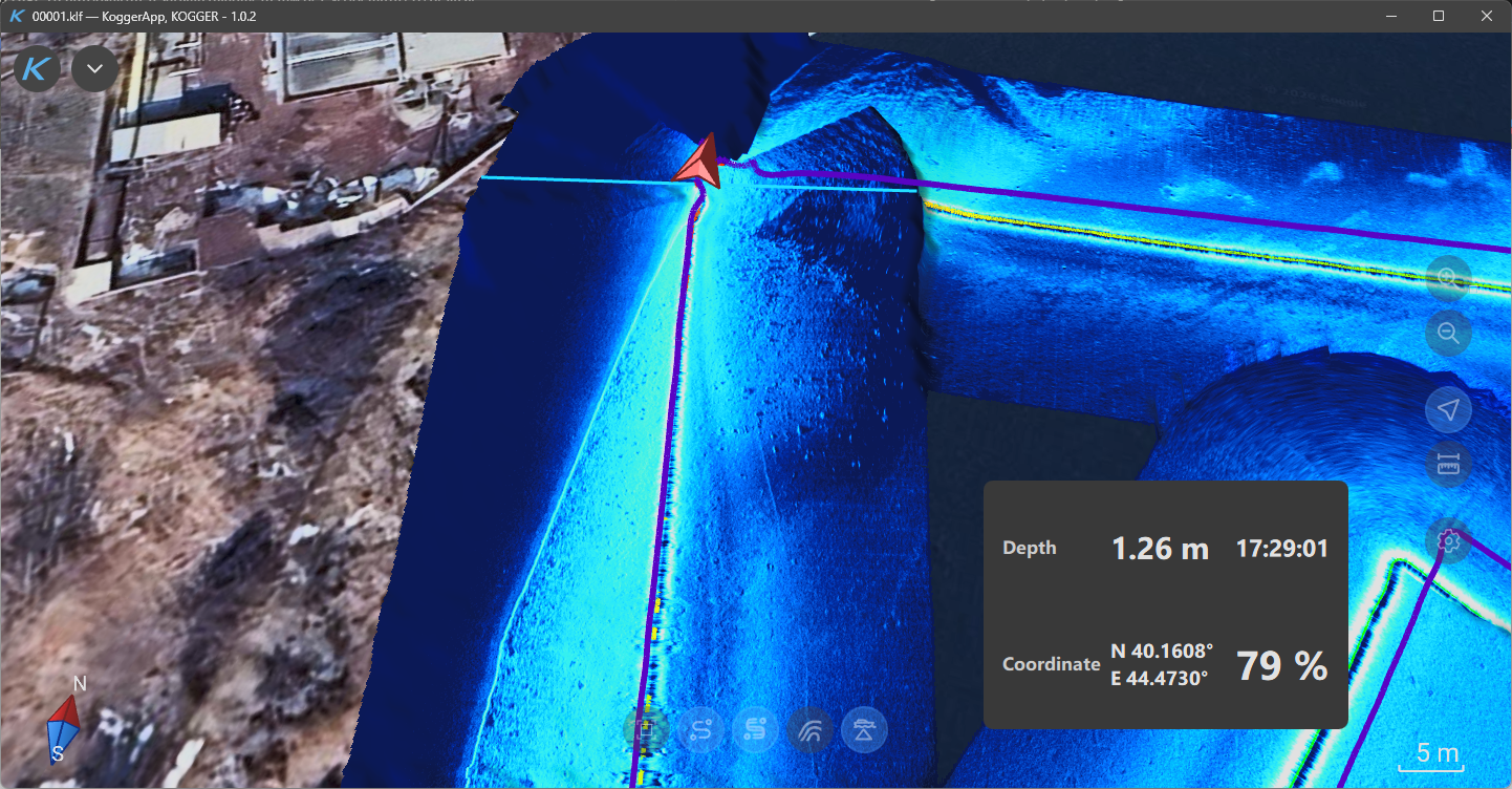
Widget panel
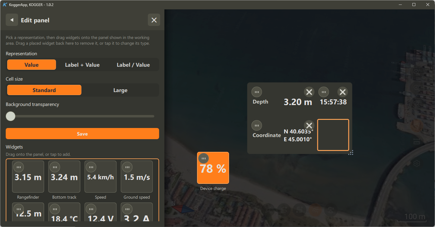
Editing a widget
Data widgets are an information layer over the scene. Whatever you need in your peripheral vision goes on it — current depth, position, speed, temperature, how much battery the vehicle has left — and everything you do not need stays off it.
They are readouts you place directly on the picture: drag them where you want them, size them to the distance you read them from. Visibility is remembered per file, so a playback session is not cluttered with fields that only mattered live.
Vehicle telemetry arrives over MAVLink, straight from the autopilot — on an unmanned boat the sonar picture and the boat’s own state sit on one screen.
Settings
The K button in the corner opens the settings, and everything the application can do is set from there.
Colour is the clearest example of how much of that is left to you. The interface has its own themes — light and dark variants, soft-contrast versions of each, and familiar editor palettes such as OneDark, Monokai, Solarized, Dracula and Nord, each with its own accent colour. The data is separate: the echogram, the mosaic, the surface and its isobaths each carry a colour scheme of their own, independent of the interface and of one another. A dark interface can sit under a light echogram and whatever depth scale reads best to you. Every picker previews the scheme as a colour strip, so you choose by looking rather than by reading names.
The same page holds the keyboard shortcuts, with a menu for the bindings themselves, and the interface language — that list keeps growing.
Whatever you set survives an update: an old installation is carried forward rather than reset.
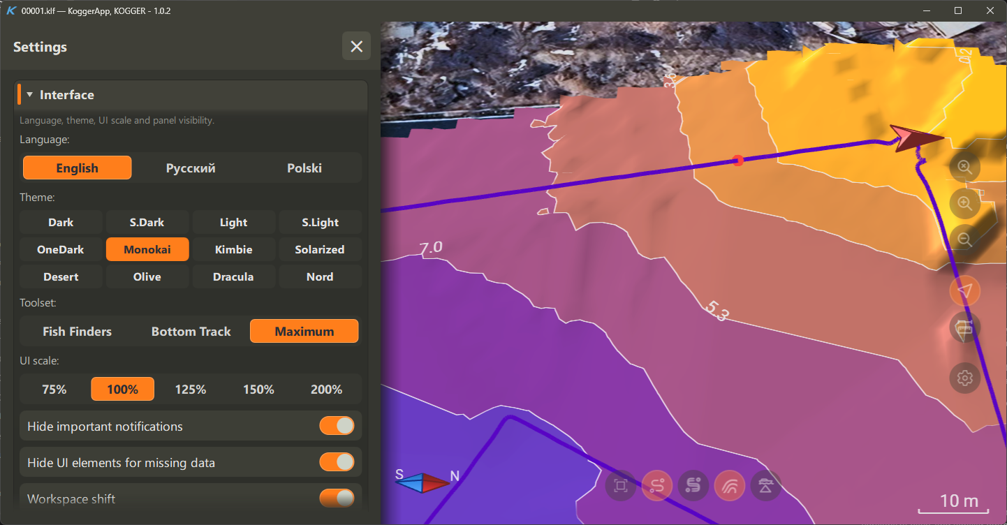
Interface settings
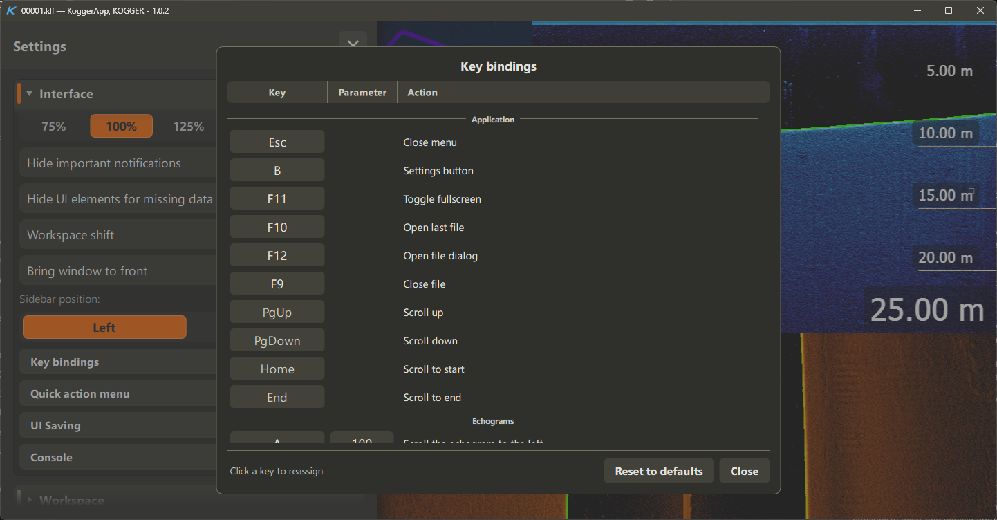
Key bindings
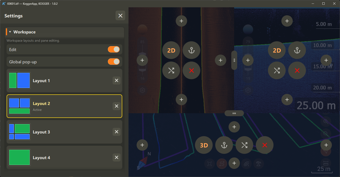
Workspace editing
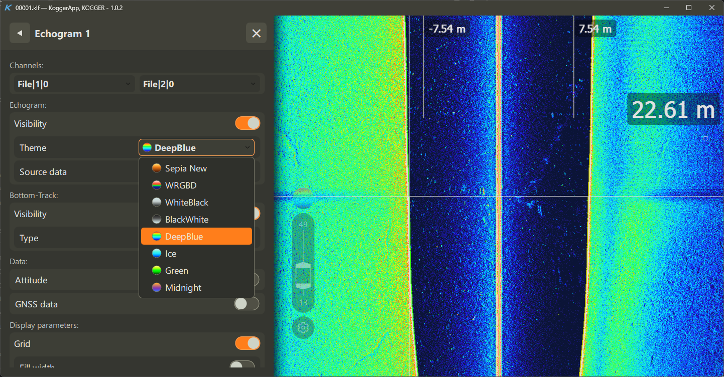
Echogram settings
Notifications and the console
Notifications arrive as toasts with per-type icons, and warnings can be muted when you already know. A notification carrying a file path opens the containing folder when you click it.
The console shows the raw conversation with the device: a configurable buffer limit so a long session does not eat memory, syntax colouring to make the stream readable, and separate toggles for NMEA and binary echo. When something behaves oddly this is the first place to look — and the fastest thing to paste into a bug report.
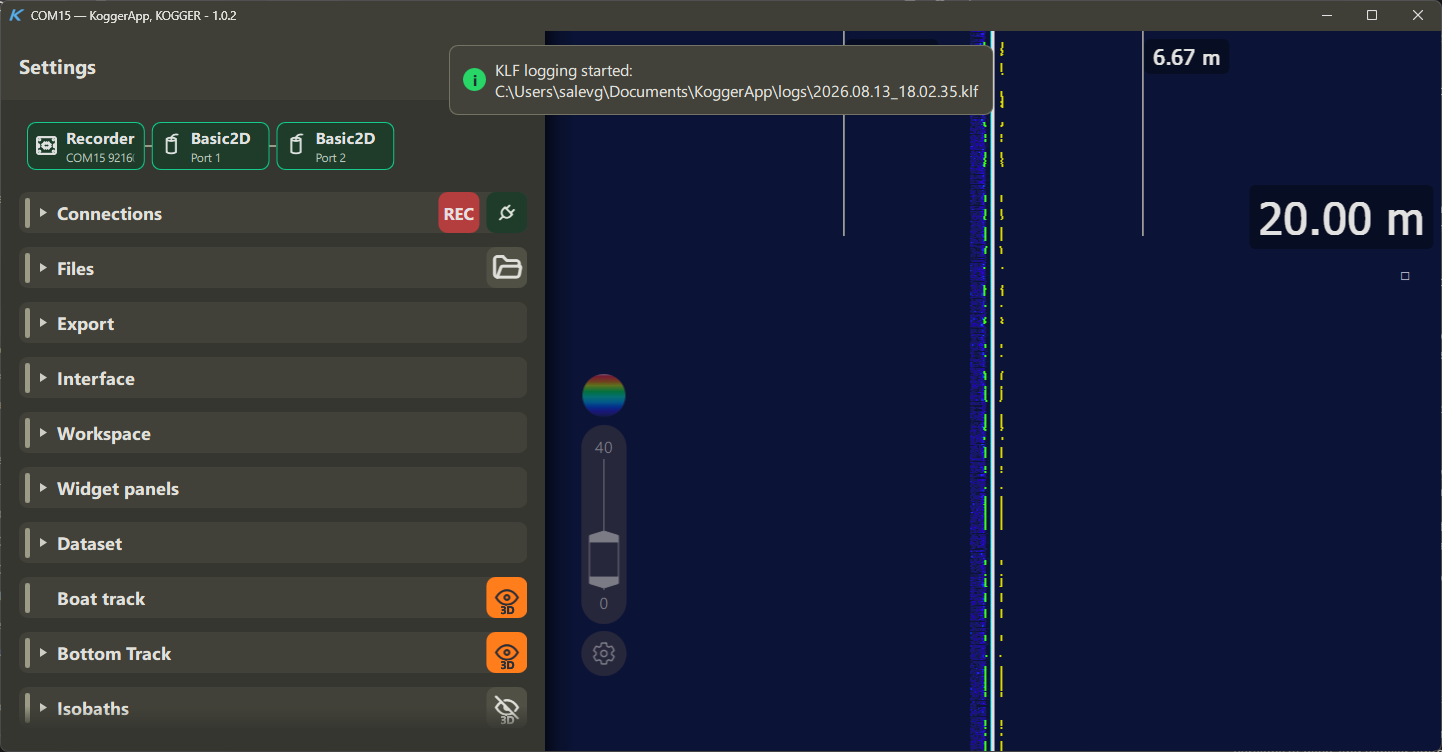
Notifications (on the top)
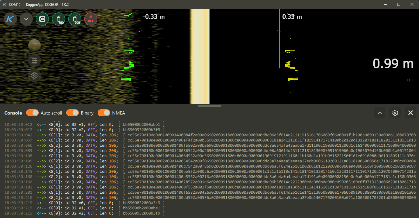
Console
Working in the 2D scene
The echogram is not only something to look at. Where the automatic bottom pick goes wrong you correct the track on the echogram itself, by hand. When something on the bottom deserves a second look you mark it as a contact and name it, and it stays with the data — including on the way out, into an export.
While data is coming in, the echogram pins itself to the end of the record, so the newest ping is the one in front of you without you asking for it.
Around that, the things you set once and forget: the loupe has its own size and magnification; the information panel on the echogram carries the fields you choose and nothing else; and each echogram keeps its own display settings, so two channels never have to look alike.
When several echograms are open they can also be tied together — the cursor on one following the others, and, as a separate choice, scroll and zoom shared across all of them. Which of the two you want depends on whether you are comparing the same moment or the same stretch of bottom.
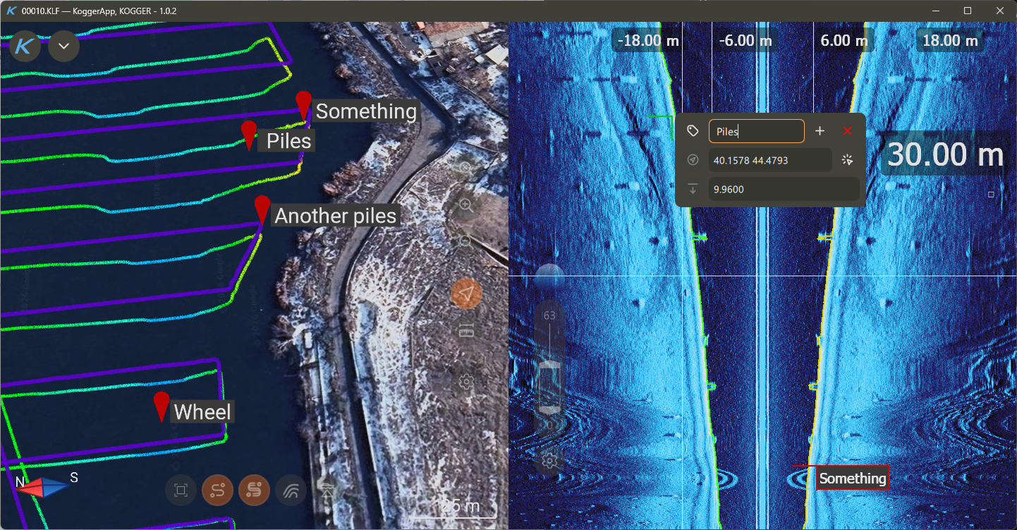
Setting up points of interest (contacts)
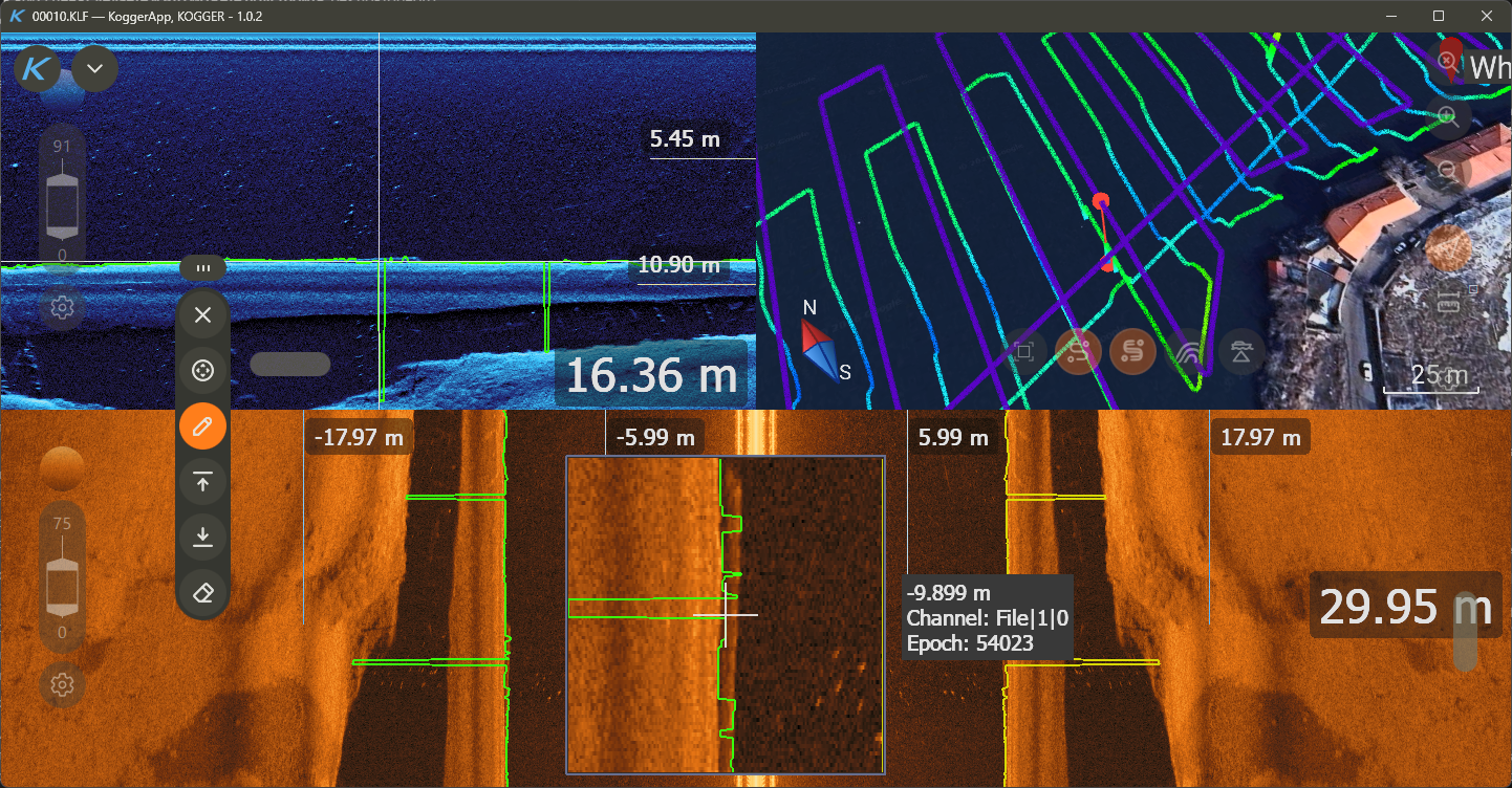
The magnifying glass tool on the echogram when manually editing the bottom track
Working in the 3D scene
The 3D scene is not only a picture either. You measure in it.
- Ruler — measure distances right on the bottom
- Scale bar — for when you have lost the sense of scale, the vertical one included
- Compass — click it to reorient instead of dragging until north looks right
- Bottom-track editing from a floating tool, so correcting the track is not tied to whichever pane holds the scene
- Cursor sync with the echogram, so a place on the 2D record and a place on the 3D bottom are the same place
The camera follows the vessel by itself — smooth, continuous tracking rather than a view that jumps to catch up — and the controls answer to a finger as readily as to a mouse.
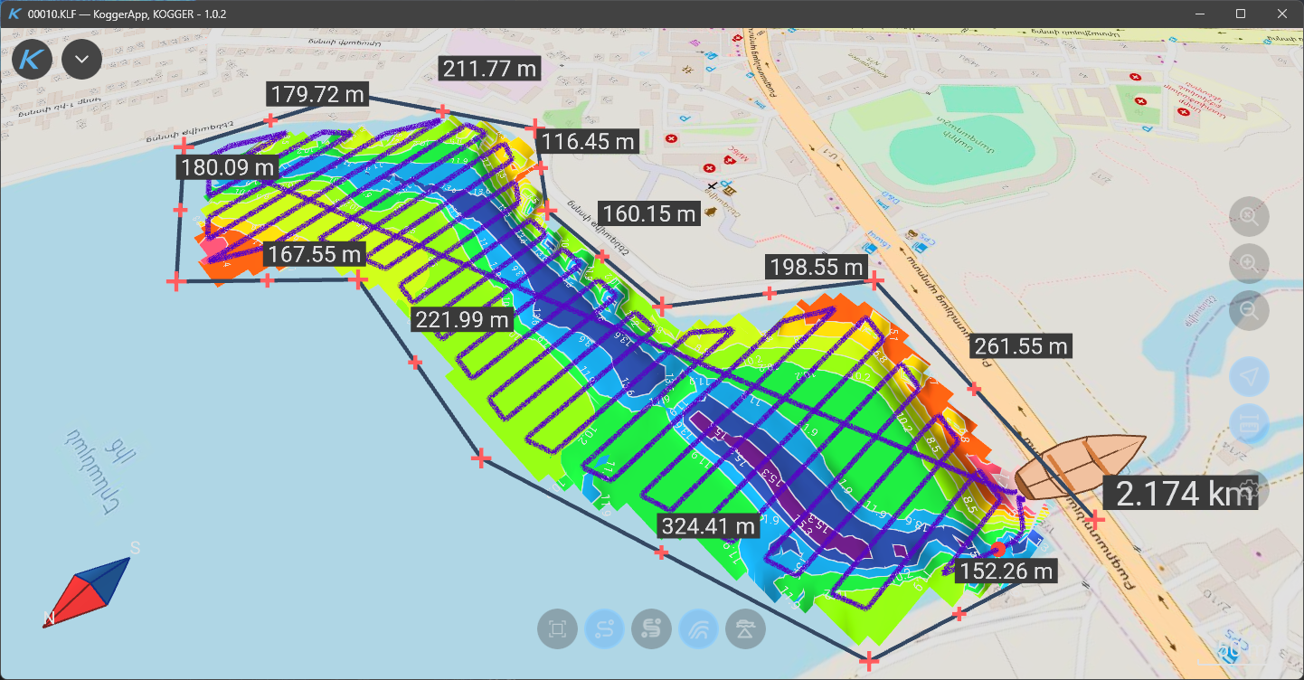
3d scene with the ruler tool
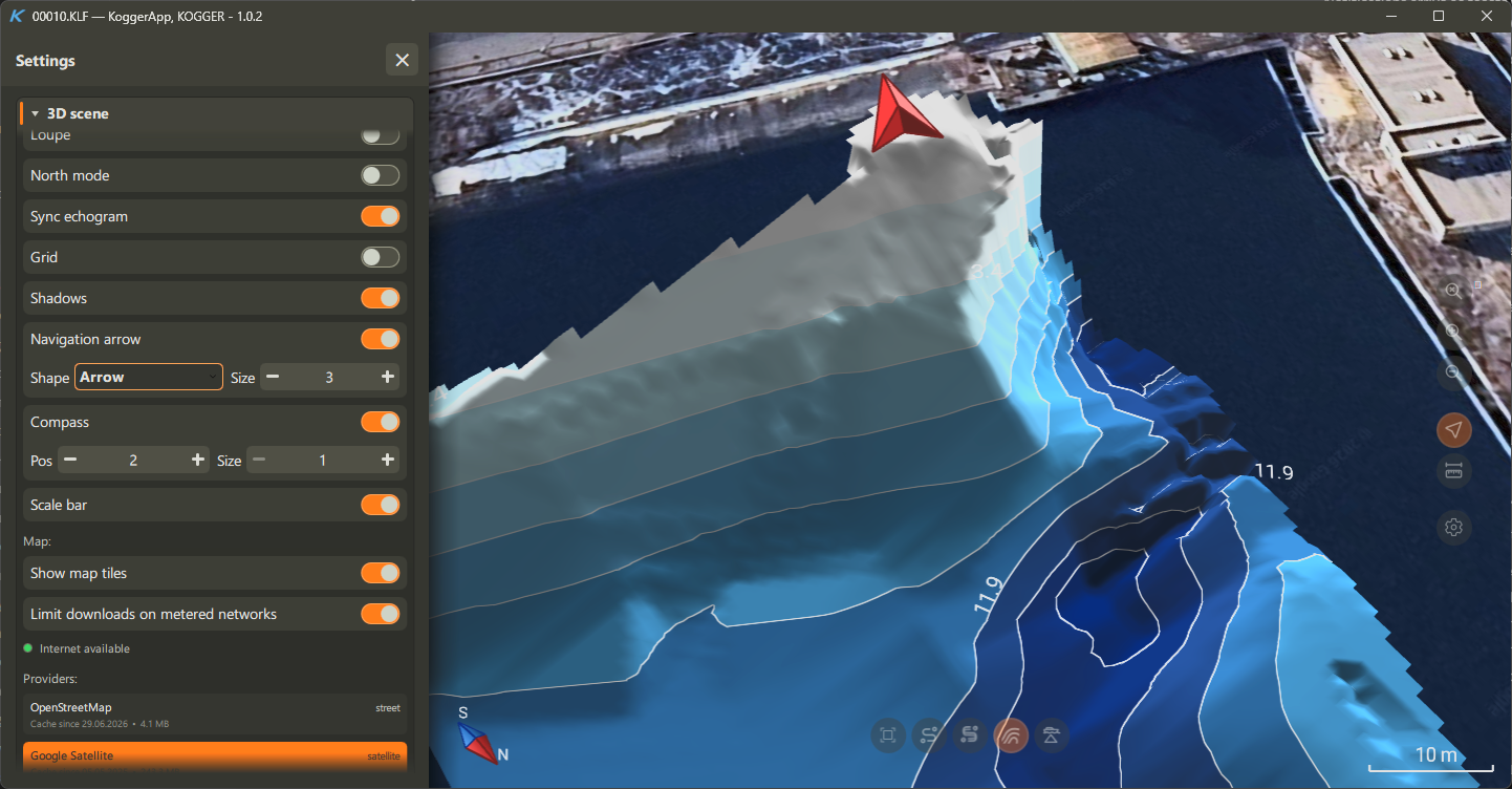
3d scene settings
What the scene shows
The scene is assembled from parts you switch on and off as the job needs: grid, boat, boat track, compass, scale bar, depth labels, shadows, the surface-quality indicator. The navigation arrow has a shape and a size of its own. North mode keeps north up if you would rather not think about orientation, and the map underneath can be shown, switched to another layer, or told to stop downloading on a metered connection.
Tuning the surface, the isobaths and the mosaic
The bottom surface is a reconstruction, and how boldly it reconstructs is your call: the depth step of the colour scale, the longest triangulation edge it may bridge, and how far it extrapolates to either side of the track. Tighten them and the surface only claims what you actually measured; loosen them and it fills the gaps between lines.
Isobaths add their own contour interval and depth labels, and their own colour scale. The mosaic has its data source, the channels that feed it, a beam angle offset for each side to match how the transducer sits, and a trace line showing where it is being built. None of it is a one-time decision — the picture is rebuilt as you change your mind.
Devices and connections
A survey starts with a link. KoggerApp talks to Kogger devices over a serial port or a TCP/UDP network, and holds several links at once — a 2D sonar and a side-scan unit on the same run, each with its own settings.
Links and the devices behind them are shown as a tree, with master and child roles worked out and labelled. On a rig where several devices sit behind one recorder, this answers what a flat list of addresses never could: what is attached to what.
- Pinned links come back between sessions, and Open last links restores the whole set you were working with. On a boat that is one tap instead of four.
- Device buttons light according to device state — a glance tells you what is connected, what is sending and what has gone quiet.
- The application header carries the connection names and the name of the open file.
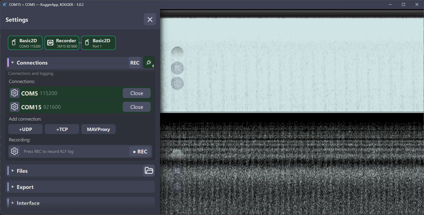
Two open connections
Device settings
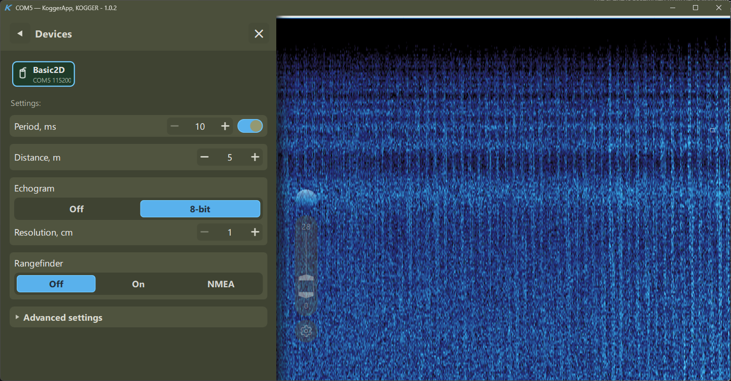
Basic2D settings
Acquisition parameters live in the application: frequency, sound speed, resolution, sampling range, pulse. Basic2D and NanoSSS each get a panel built around the way you actually change things — the sample count recalculates when you change resolution, distance runs on a progressive scale, and the parameters you touch once a season sit below the cut instead of crowding the ones you touch every hour.
Profiles
A profile is a saved set of sonar settings. Pick one and the whole set is written into the device — no walking through parameters one at a time. Shallow harbour work in the morning and open water in the afternoon become one tap apart.
The recorder
A recorder on the boat keeps writing whether or not a laptop is attached. KoggerApp reads its archive directly: refresh the list, see what is on the device, download what you need, re-download anything that arrived damaged, import a file into the current session.
The status panel is the part that matters in the field. It tells you which log is being written and how many devices are feeding it, how much space is left, and — the message you actually want — when a source has gone silent and nothing is being recorded at all. A recorder that quietly stopped is the worst thing to discover back at the office.
Sonars attached to a recorder can also be driven from a shared timer, so several units on one rig ping in step instead of talking over each other.
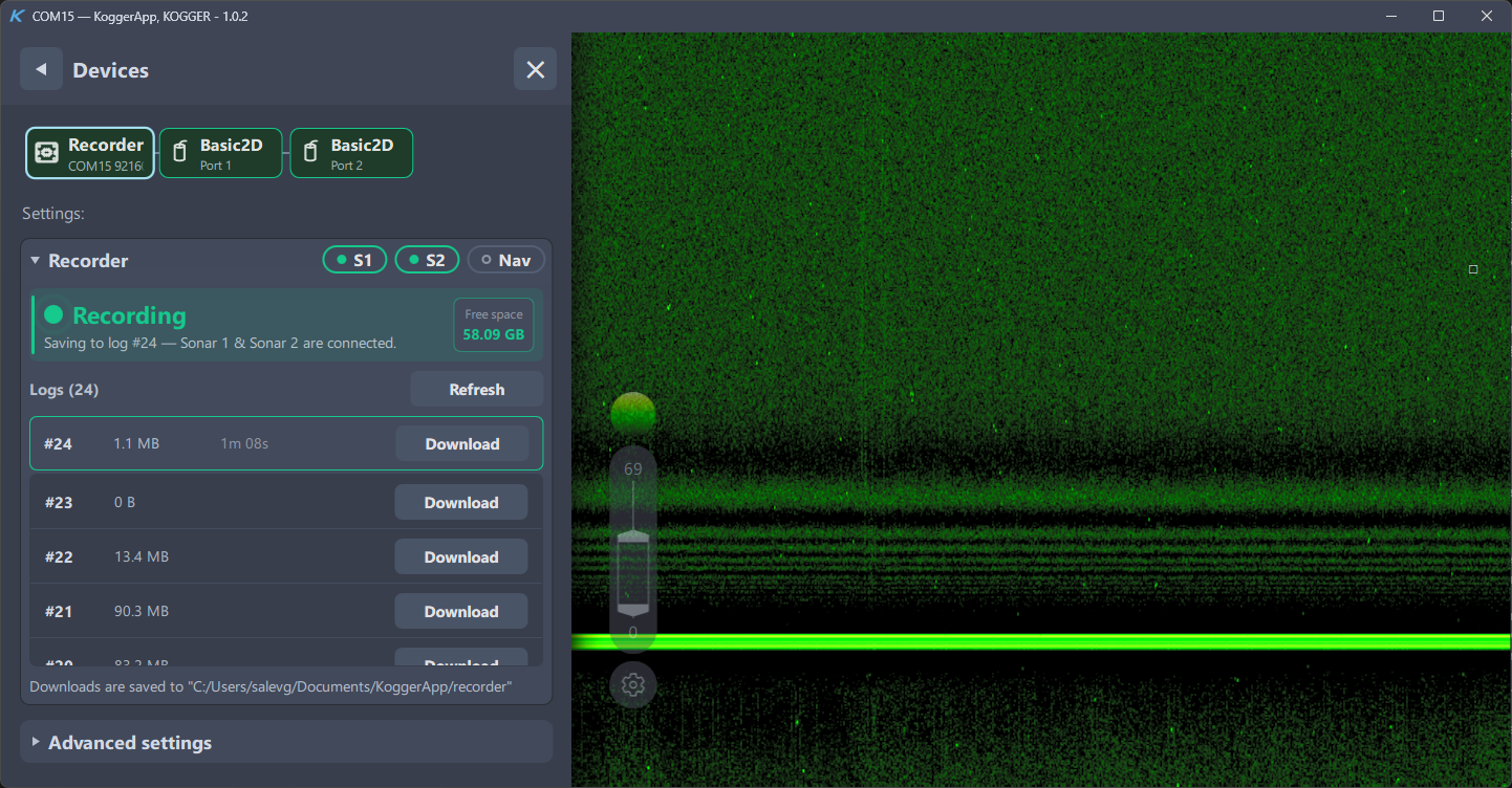
Recorder settings
Logging to the laptop
Recording locally works the same way from the application side, and the notification tells you the full path the log is being written to — so the file you just recorded is one click away rather than somewhere in a folder tree.
Files and export
Nothing has to be connected. A recorded file opens into the same views and the same tools as live data.
Opening
KLF is the application’s own log format; the Windows installer can associate it, so a log opens by double-click. XTF opens too — a third-party side-scan record lands in the same views as your own data. There is a recent-files list, and you can drag a file onto the window.
Exporting
- XTF — hand the survey to any package that reads side-scan
- CSV — the general-purpose route into GIS, CAD and spreadsheets
- Complex signal to CSV — raw signal out, for anyone doing their own processing
- Surface to CSV — the triangulated bottom surface
- UI state to JSON — the whole interface: layout, panels, every echogram and 3D setting
The export folder is set once and used by everything.
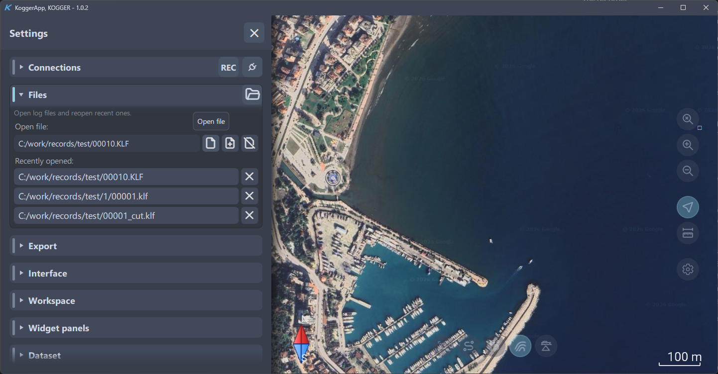
Open log file
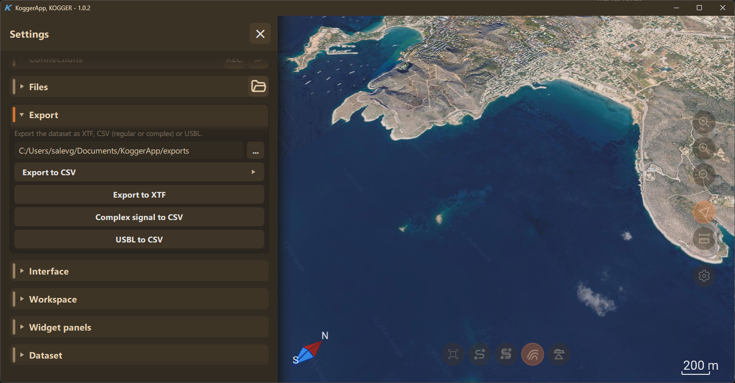
Export menu
Choosing what goes into the CSV
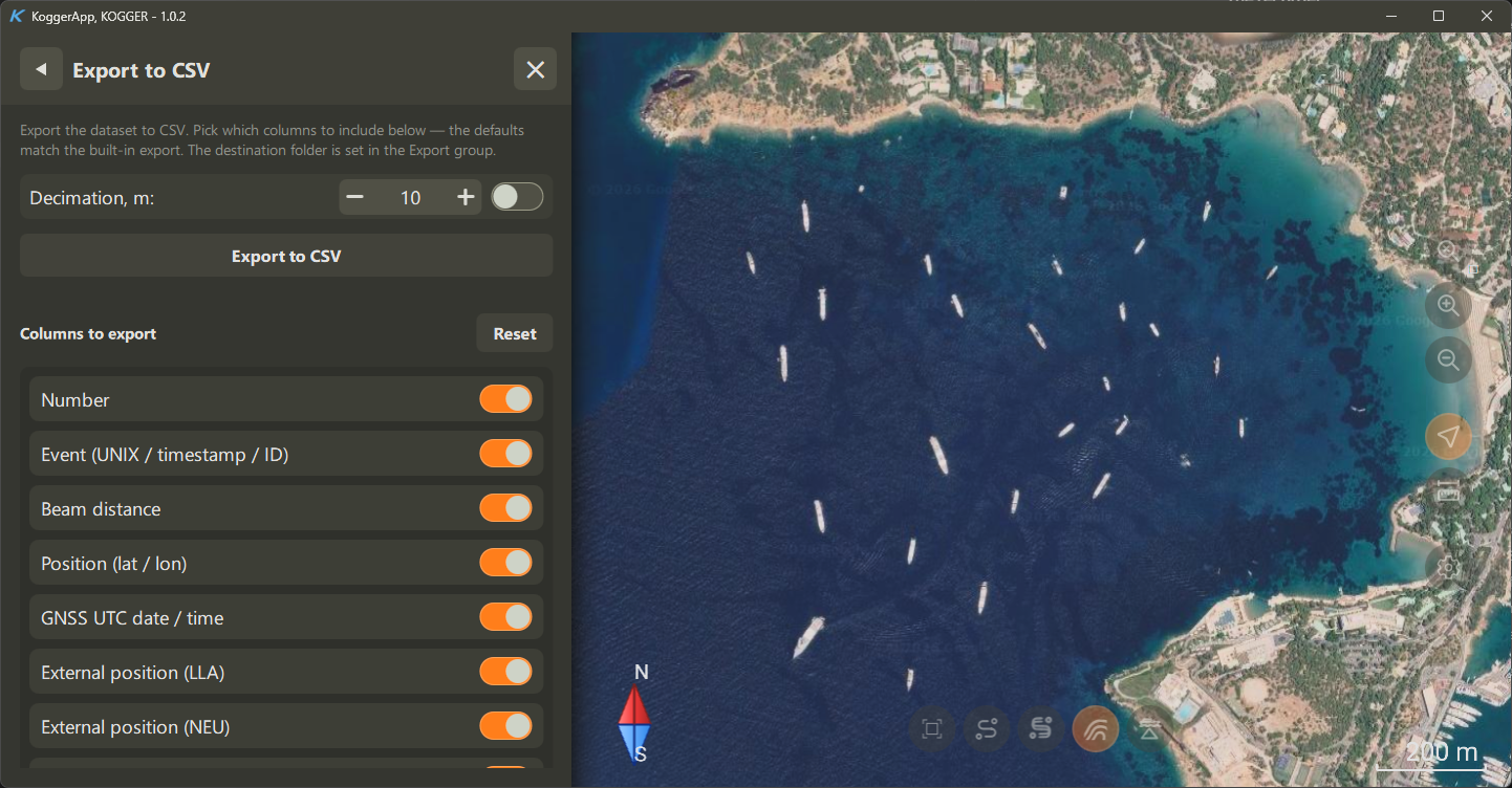
Selecting CSV export fields
The CSV is not a fixed dump. You pick the columns: measurement number, event columns, GNSS date and time, position, external position in LLA or in local NEU, rangefinder distance, post-processing distance, beam distance, bottom height, absolute heights of the bottom and of the sonar, contact title and distance.
There is also decimation — keep one point per given distance interval, or leave it off and export every point.
Carrying the setup with you
Exporting the UI state writes your whole arrangement to a single file. Set the application up on the office machine, carry the file to the boat laptop, import, and everything is where you expect it.
That is the rest of the application: a workspace you arrange once and recognise every time, a scene you can measure in, devices that tell you what they are doing, and files other tools accept.
The first post, on the echogram, the bathymetric surface and the side-scan mosaic, is .
Happy surveying!