
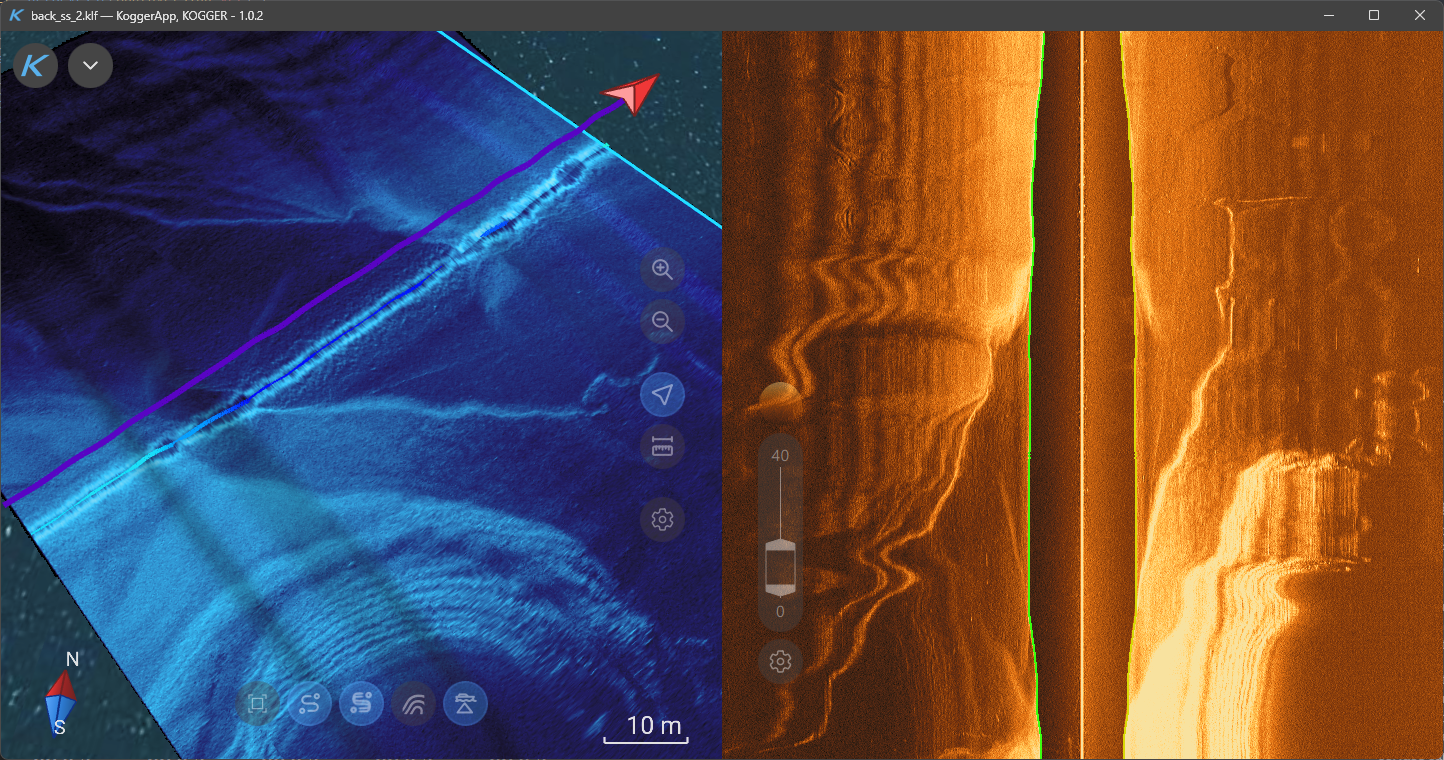
Echogram and side-scan mosaic on one screen
KoggerApp is the software half of a Kogger sonar: free, (GPL-3.0) sonar survey software for Windows, Linux and Android. It connects to Kogger devices over serial or a TCP/UDP network — several at once — configures them, and turns what they return into something you can read while you are still on the water.
That data gets three live views: an echogram of the water column and bottom returns ping by ping, with depth picked from it and correctable by hand; a 3D bathymetric surface with isobaths recalculated as you survey; and a side-scan mosaic stitched and georeferenced in 3D. All three sit over a globe map, and the results can be exported for use in other tools.
Around them: sonar, navigation and autopilot telemetry, log recording and playback, acquisition parameters, and a workspace you arrange yourself.
More on the ; the latest build is on the .
1. Echogram
The echogram is the first thing you watch. It draws the water column and bottom returns ping by ping, in real time from a connected sonar or from a recorded file.
- Colour scheme switcher and brightness slider on the echogram itself, where you need them, rather than in a settings page
- Live scrollbar
- Loupe with a live preview, on every echogram
- Contacts — mark a target, edit it, and open it from a contact pop-up
- Rendering modes — Raw, Side-Scan and TGC, with time-varied gain controls in the settings page
- Adaptive controls. Controls hide when the data behind them is absent, so a single-channel file shows no multi-channel machinery.
- The echogram view comes back with the session
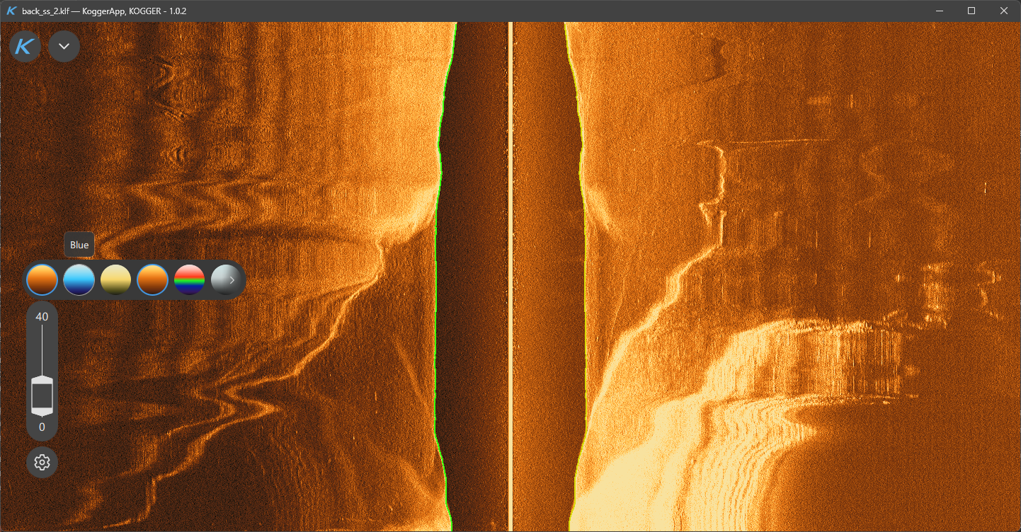
Echogram and color scheme change widget
Depth and bottom track
Depth comes from the sonar data. The bottom-track detector is configurable — presets for Normal 2D, Narrow 2D and Side-Scan, plus threshold, gain slope, vertical gap, horizontal window, min/max range and the sonar offset in XYZ. Where the automatic pick is wrong, you edit the track by hand, either on the echogram or with the global editing tool in the 3D scene.
Synchronization across views
Two independent sync modes across 2D views:
- Cursor / time sync — moving the cursor on one echogram moves it on the others, with offset accounting between channels
- Independent vertical-view sync — depth ranges track each other while horizontal positions stay separate
A configurable info plate on the echogram shows the values you select; the slave echogram in sync mode shows a reduced set.
Vertical orientation
The echogram runs vertically, with contacts, loupe and info overlays adapted to that orientation.
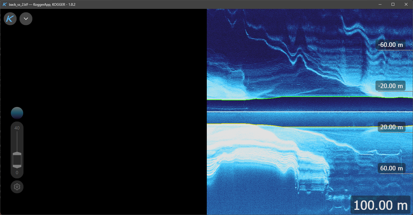
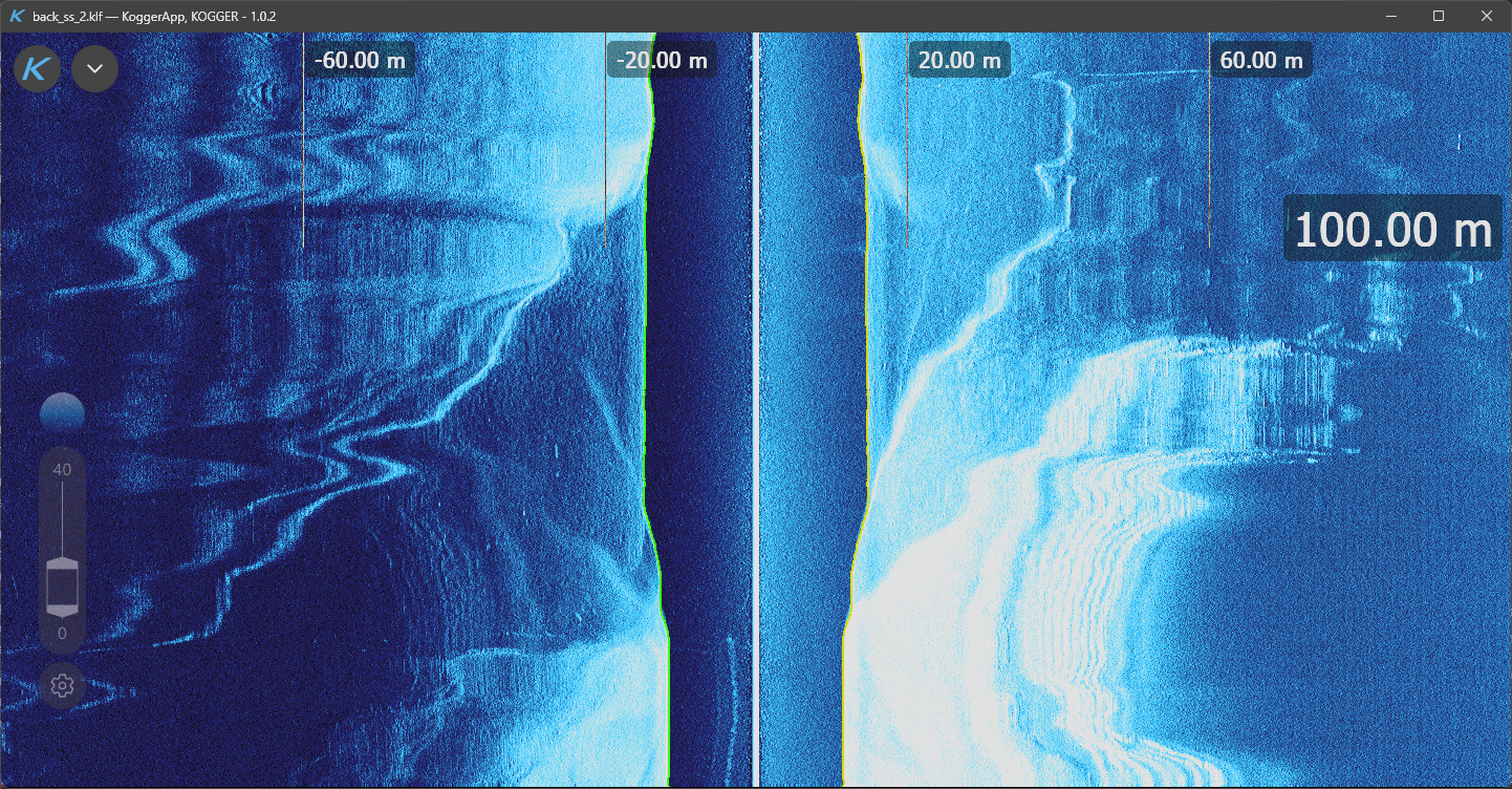
Horizontal/Vertical display of the echogram
2. Bathymetry: the 3D bottom surface and isobaths
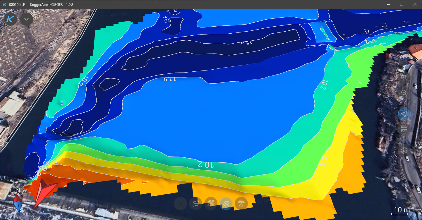
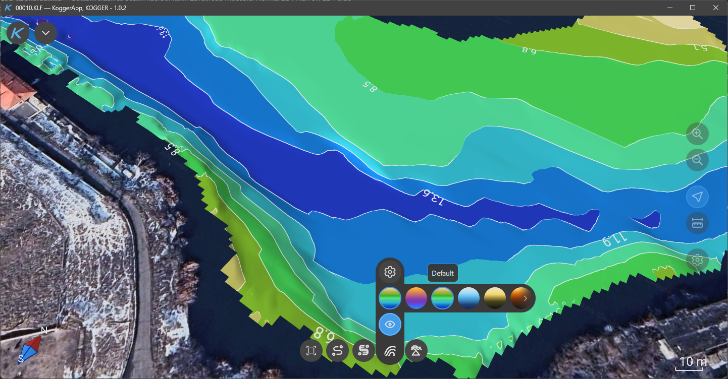
Surface with isobaths (change of color scheme)
Bottom-track points become a triangulated bottom surface in the 3D scene, coloured by depth, and the surface rebuilds incrementally as new points arrive — the picture fills in during the run rather than after it.
Isobaths are equal-depth contour lines on that surface. Depth labels run along the lines, and thin out where they would collide. The contour interval is yours to set, as is the colour ramp: a choice of palettes by depth.
Three controls shape the surface itself:
- Step — the depth quantization of the colour scale
- Edge limit — the longest triangulation edge allowed, which stops the surface from bridging across gaps between survey lines
- Extra width — how far the surface is extrapolated to either side of the track
You can export the finished surface.
3. Side-scan mosaic in 3D
The side-scan mosaic builds in real time. Each ping contributes its left and right swaths, referenced to the boat position and heading, and The application rasterizes those amplitudes a georeferenced bottom image and lays it over the 3D surface. What you get is not a flat strip chart but the bottom itself, in place, growing as you survey.
The mosaic and the bathymetry from the previous section are not two separate pictures. The mosaic traces onto the same triangulated height mesh, so the image follows the relief instead of lying on a flat plane — a slope reads as a slope, and a depression carries its texture down into it. Heights from the triangulation take priority. Where the triangulation has no data yet, the mosaic contributes heights of its own from the depth measured on each ping. The two feed the same surface, and the result looks like the bottom rather than like an image of it.
- Data source — Raw, Side-Scan or TGC
- Channel selection — which channels feed the mosaic, or all of them
- Beam angle offsets for the left and right sides in degrees, to compensate for how the transducer is mounted
- Trace line — shows the line the mosaic is currently being built along
- Palettes — a choice of colour ramps for the mosaic image
The mosaic and the isobaths share the same surface, so they are mutually exclusive: turning the mosaic on hides the contour lines.
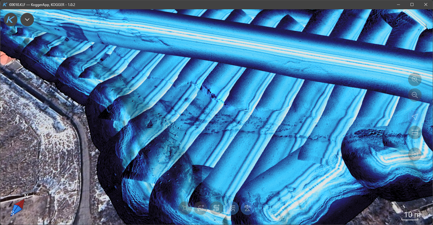
3D side scan mosaic
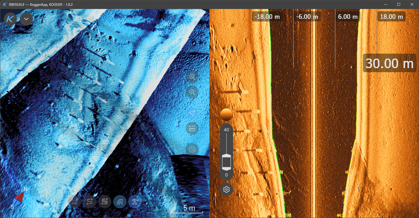
3D side-scan mosaic synchronized with the echogram
4. Maps and georeferencing
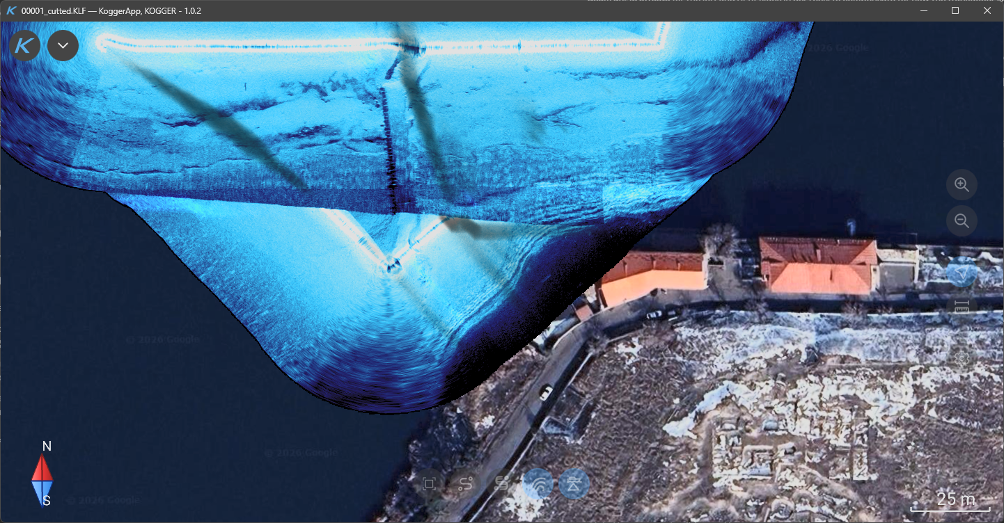
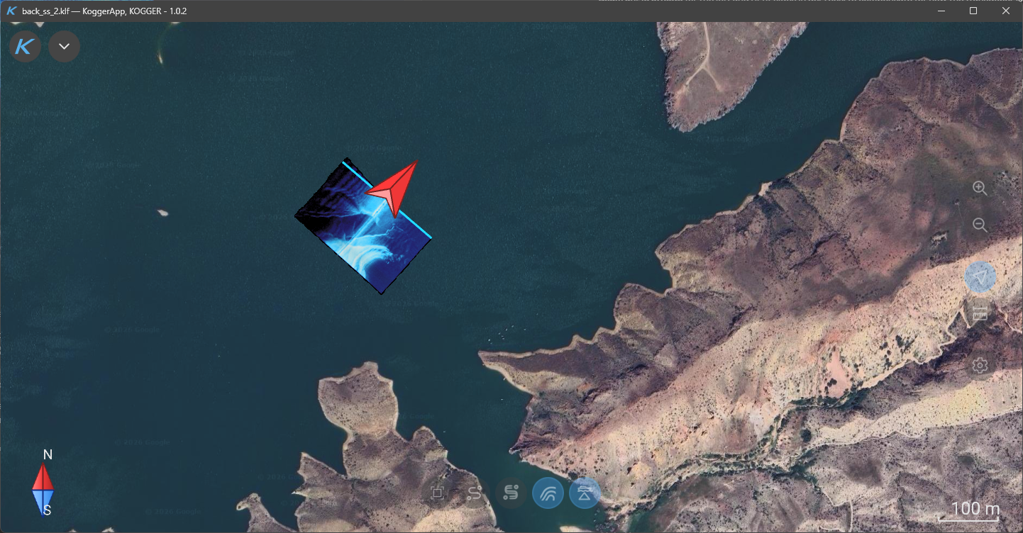
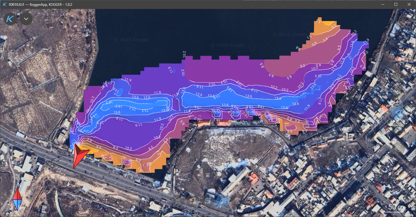
Various representations with reference to the map
Under the surface and the mosaic sits a globe map that ties a survey to its location.
The application caches tiles locally, and the settings page shows what each layer has already stored, so you know what is available without a connection. On a metered connection the application can hold off downloading tiles rather than spending your data plan on map coverage.
Those are the main things the application does. The rest — the workspace, working in the 2D and 3D scenes, devices and connections, files and export — is in the .
Happy surveying!